|
|
| Impressum | Copyright © Klaus Piontzik | |
| German Version |
5 - The approach for the basic field
5.1 - Basic oscillations
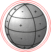
| On account of the previous consideration the
conclusion lies near that the magnetic field of the earth
owns a symmetrical structure with regard to a three-axle
ellipsoid. In this structure appear certain angles which
are integer parts of 360 degrees. If one looks away from the real field-generating elements in the earth inside and concentrates merely upon the external field reaching round the earth, so it allows the following approach: The whole field of the earth can be explained, after the Huygens principle (Huygens - Dutch physicists, in 1629-1695), by using a spectrum of discreet frequencies and worldwide fixed "source points". Namely as a sum of an assemblage from standing spatial waves, the so-called basic oscillations (elementary waves). These spread from the "source points", and induce by superposition of all oscillations - as a steady state - the earth field. |
| The
beginning occurs on the base of oscillations on or around
a ball Examples of oscillation possibilities: |
 |
 |
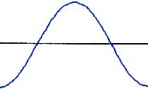 |
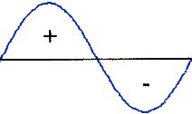
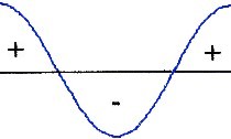
| Sine | Cosine |
| Sine or cosine = oscillation = wave |
| This is
valid for physical oscillations: Formula: f·λ = c (frequency multiplied with wavelength is equal to speed of light) |
5.2 - The theorie
| To determine the real source points of the field and the basic oscillations, it requires, as already mentioned, a two-dimensional fourier analysis (see chapter 8). The illustration with a qualitative attempt however at first is enough here: | ||
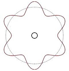 |
Visualise a
sphere, around a standing wave has established. By
analogy to the Bohr nuclear model, if one understands the
running electron around as a wave by De Broglie. Then merely an integer number of oscillations fits round the whole circumference.. n · λ ∼ 360° = 2π |
|
| Illustration 5.1 - basic oscillation | ||
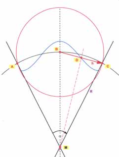 |
The wavelength is proportional to the angle
Alpha: λ ∼ α |
|
| Illustration 5.1.1 - basic oscillation and angle |
| Condition for n oscillations around a ball: | n · α = 2π |
| A standing wave around a ball can be
interpreted physically as a steady state
A ball owns 3 degrees of freedom Only for
illustration: As a source point serves the North
Pole (picture 5.1). If one lets proceed the basic
oscillation from North Pole through South Pole again run
to the North Pole, the second wave arises around the
equator. For these first both oscillations exists a
mathematical draught, that is suited for a
representation, namely the spherical harmonics. |
5.3 - Spherical harmonics
| Standing
waves on a ball surface are called spherical
harmonics. There exist 3 kinds of oscillation
forms.
(See also Torges „Geodäsie", page 41-43.) |
||
 |
Zonal
spherical harmonics depend merely on the degree of
latitude sin φ cos φ |
|
| Illustration 5.2 - Zonal spherical harmonics | ||
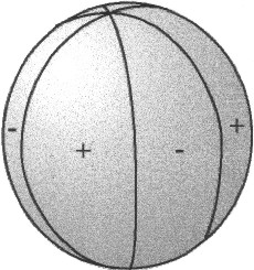 |
Sectoral
spherical harmonics depend merely on the degree of
longitude sin λ cos λ |
|
| Illustration 5.3 - Sektoral spherical harmonics | ||
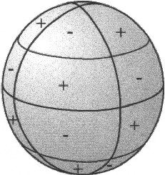 |
Tesseral
spherical harmonics depend on the degree of latitude and
on the degree of longitude sinφ·sinλ sinφ·cosλ cosφ·sinλ cosφ·cosλ |
|
| Illustration 5.4 - Tesseral spherical harmonics | ||
5.4 - Addition of sine waves
| Spherical harmonics can be explained as two sine - or cosine waves which stand vertically on each other and mutually interference themselves. Two such waves can be added according to the following qualitative rules: | ||
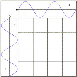 |
The zero points of both waves are transfered on the consideration level So the the zero grid occurs. | |
| Illustration 5.51 Zero-Grid from two sine waves | ||
 |
1) + and + produces + 2) - and - produces - 3) + and - produces 0 As to be seen, fields with different
algebraic signs produce respectively different states.
There exist three oscillation states: |
|
| Illustration 5.5 - Addition of two sine waves | ||
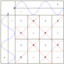 |
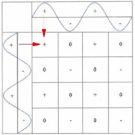
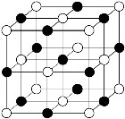
It is striking that all
zero fields lie diagonal to each other.
If one connects now the zero fields with each other, the
accompanying picture 5.6 arises. In the farther course this grid-like (red) oscillation structure is called basic field. Then the producing (blue) sine waves are called basic oscillations. |
|
| Illustration 5.6 - Origin of the basic field | ||
5.5 - The basic field
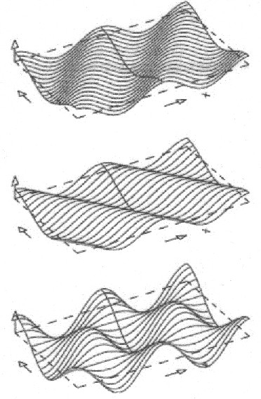
| If one interferences two sine waves, which stand vertically on each other, quantitatively so the illustrations 5.8 and 5.9 arise. Clearly is to be seen the exact grid forming, as well as the alternate polarity of the single fields. |
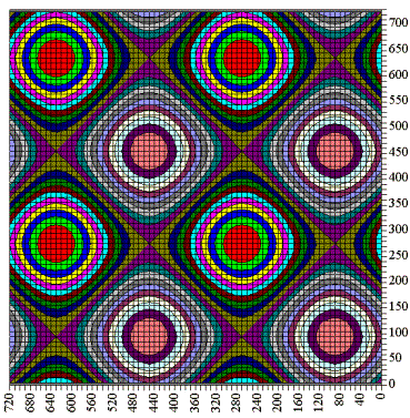 |
The superposition of two - vertically on
each other standing - waves produces the known grid
pattern with the alternate polarities of the grid fields.
(Illustration 5.8 and 5.9) Here is seen that the field maxima appear as point-shaped in the middle of the squares, while the lines consist of zero values - by analogy to the Chladni-sound figures. |
|
| Illustration 5.8 - The basic field | ||
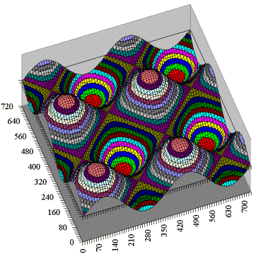 |
Mathematical
seen basic fields or tesseral spherical harmonics can be
explained by the multiplication of two
sine or cosine waves. It originate in such terms how they appear in the equation by Gauß and Weber (chapter 2.7). See also chapter 10.3 |
|
| Illustration 5.9 - The intensity of the basic field by 3D view | ||
| basic field = grid = two-dimensional oscillation structure |
| Well is
also to be seen in illustration 5.9 that in each case two
generated grid fields again prove a (generated)
oscillation. This permits two views of the grid: 1) The generated
grid is described in the level of the basic oscillations |
| Possibly still a second grid cam be marked here. Namely the maximum grid: It connects the field maxima (minima) with each other and shows the extremalen course of the field. |
| Because a complete square grid on the surface of a sphere cannot be realised, so the oscillation systems are formed like the geographic grid system. There always exist two poles. Then the accompanying meridians and circles of latitude form the grid system. |
| Pictures on radar base, which show unambiguously basic fields or tesseral spherical harmonics on the solar surface, have originated from the solar satellite Soho. There the question arise whether the magnetic field of the earth also such oscillation structures has produced. |
| In the beginning of the 50s last century Dr. med. Ernst Hartmann described a grid system which proceeds in the magnetic north-south-direction. This Hartmann-grid is treated in the chapter 11 more in detail. With the basic field model an attempt is given to describe the Hartmann-grid as a magnetic tesseral spherical harmonic. |
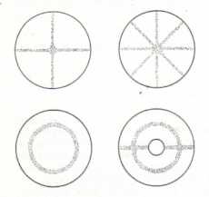 |
The Chladni-sound
figures form an Analogon here. If one irradiates
a sandy coated metal plate with sound waves, standing
waves on the plate ocurrs in the resonance case. Then
along the zero values the sand remains lying and the
typical oscillation figures appear. (see also: „Physik" from Gerthsen, Kneser, Vogel – chapter 4.1.5 – Eigenschwingungen deformierbarer Körper) |
|
| Illustration 5.7 - Chladni - Figures |
| The superposition of two sine waves can be shown three-dimensional also like in illustration 5.10: |
|
| Illustration 5.10 - Basic oscillations and basic field |
| While the mathematical concept of the spherical harmonic does not ask for the cause of the oscillation field, the underlying waves must be incorporated in case of the physical consideration. The concept of the basic field performs this. The basic field is defined by the basic oscillations. |
| The term basic
field is as a physical equivalent to the concept of the mathematical tesseral spherical harmonic |
Tesseral sherical harmonics = Product of two oscillations = 2 vertically waves standing on each other = grid = basic field = two-dimensional oscillation structure |
5.6
- Huygens Principle
(in addition
to the book)
| After chapter 5.2 a ball owns 3 degrees of freedom. 2 degrees of freedom would be covered by the use of spherical harmonics. The third degree of freedom is still absent: the radial direction. In addition the understanding of a physical representation is required, with which the expansion of physical waves can be described: the Huygens principle. |
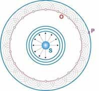 |
The Huygens principle goes out from a source
S, which generates uniformly wave fronts in all
directions. To receive the resultant wave front in the point P, however, it is not necassary to look the whole propagation from S. |
 |
The Huygens principle says
that every point (O) of a wave front can be looked as a
starting point of a new wave, the so-called elementary
wave (grey). The situation of the resultant wave front (P) arises by overlapping (superposition) of all elementary waves |
| The wave origins (O) deliver by superposition of the elementary waves the resultant wave front (P). In three dimensions elementary waves are spherical, in two dimensions circularly. |
 |
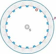
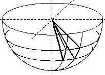
wave around a ball: extrema of the wave = source = wave origins 1 oscillation = 2 sources |
 |
Oscillation state for one
oscillation after the Huygenschen principle with a maximum (wave mountain) as
a source (green) Besides, the minimum fronts (blue) and the maximum fronts (red) are the elementary waves |
| In the previous picture the oscillation situation is shown in the cross section for one oscillation. In the following picture the oscillation situation is shown for n oscillations. |
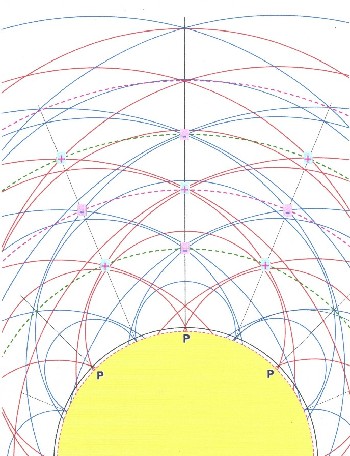 |
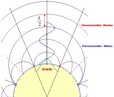
Going out from the source points P,
after the Huygens principle, around
every source point arises concentric circles (elementary
waves) of minimum zones (red circles)
and maximum zones (blue circles). Because a stationary state exists, the wave fronts are stationary in the spatial situation. The superposition of the elementary waves occurs according to the same rules like already in chapter 5.4 described. |
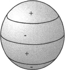
| From the
interference overlapping of positive wave fronts arises Oscillation
maxima (with plus marked) and in the following
as positive poles called From the interference overlapping of negative wave fronts arises Oscillation minima (with minus marked) and in the following as negative poles called namely where several wave fronts form an intersection or an area of concentration By the superposition of positive and negative elementary waves also form zero Pole The oscillation extrema, resulted by the superposition, lie again on ball surfaces which the generating ball (e.g., the earth) sketched concentrically, in the following layers = L called Between these extreme layers exist zero Poles which also lie on concentric ball bowls - in the following zero walls called |
 |
It turns out this simplistic view of the
resultant field: black sketched lines = extreme lines = layers magenta lines = zero lines = zero walls The generated layers L form a radial standing wave |
| The mathematically, physical inquiry of the layers, also the quantitative regulation, occurs in Kapitel 12 |
5.7
- Stratification structure, oscillation structure
(in addition
to the book)
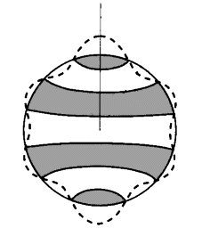
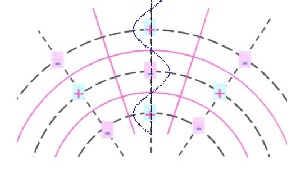
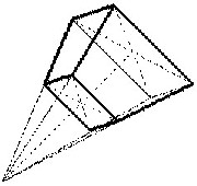
| One standing wave on a ball generates a rotation-symmetrical spatial structure: |
 |
|
| The poles lie circularly
on concentric balls The zero walls form concentric cones and concentric balls |
 |
| Stratification structure = from one standing wave generated radial stratification structure |
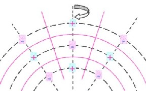
| Two standing waves on a ball generate a radial grid-shaped structure: |
 |
 |
 |
| There arise two view possibilities: |
| The zero surfaces form the
walls of a grid-shaped radial oscillation system The poles lie in the centre of the zero cube |
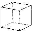 |
| The poles also form a
grid-shaped radial oscillation system like a molecular
grid (e.g., NaCl) in the following pole grid
called The pole connections behave like sticks which swing at both ends freel |
 |
| Space grid = from two standing waves generated radial stratification structure |
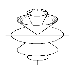
| Oscillation structure = sum of all possible space grids around a ball |
| Remark: The stratification structure generated by one wave is identical with the stratification structure that two waves generate. |
![]()
| The book to the website - The website to
the book at time is the book only in german language available |
||
|
|
| The Advanced Book: Planetary Systems |
| The theory, which is developed in this book is based on the remake and expansion of an old idea. It was the idea of a central body, preferably in the shape of a ball, formed around or in concentric layers.
Democritus was the first who took this idea with his atomic theory and thereby introduced himself to the atoms as fixed and solid building blocks. Is the atom used as a wave model, that allows to interpret concentric layers as an expression of a spatial radial oscillator so you reach the current orbital model of atoms. Now, this book shows that these oscillatory order structures, described by Laplaces equation, on earth and their layers are (geologically and atmospherically) implemented. In addition the theory can be applied on concentric systems, which are not spherical but flat, like the solar system with its planets, the rings that have some planets and the moons of planets or also the neighbouring galaxies of the milky way. This principle is applicable on fruits and flowers, such as peach, orange, coconut, dahlia or narcissus. This allows the conclusion that the theory of a central body as a spatial radial oscillator can be applied also to other spherical phenomena such as spherical galactic nebulae, black holes, or even the universe itself. This in turn suggests that the idea of the central body constitutes a general principle of structuring in this universe as a spatial radial oscillator as well as macroscopic, microscopic and sub microscopic. |
|
![]()