|
|
| Impressum | Copyright © Klaus Piontzik | |
| German Version |
9 - Evaluation of the fourier analysis
9.1 - The static part
| According to the fourier analysis the static part of the earth field amounts to 47,2183 μT. The most minimum value of the field lies at 24 μT, the most maximum value amounts to 62 uT. This declares that about 75% of the field behave like a permanent magnet. |
9.2 - The zonal part
| The zonal part of the field originates from the evaluation of the averages in the fourier analysis. It contains terms that are only dependent from the latitude φ (Phi) and can be shown as follows: |
 |
In the
Illustration 9.1 is to be seen which forms a maximum
zone, namely with φ=75 degree round the North Pole. About 2.8 degrees below the equator there is a minimum zone. And exactly on the South Pole one receives one more maximum point. With thus the zonal field is based primarily on the oscillation of the number 2. Conditioned by the term 11,3642·cos2φ, which puts out the biggest portion in the zonal field. That gives the field, together with the permanent part, then also a character similar to a dipole. |
|
| Illustration 9.1 - Zonal part of the magnetic field |
9.3 - The sectoral part
| The sectoral part of the field originates from the evaluation of the constant limbs in the tesseral portion from the fourier analysis. It contains terms that are only dependent from the longitude λ (Lambda) and can be shown as follows: |
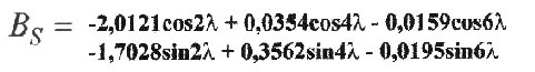 |
 |
In the
Illustration 9.2 is to be seen which forms a maximum
zone, namely with the longitude λ =-83,5 degree of west and λ=96,5 degree of east beside the small ellipsoid axis. The minimum zones lie with longitude λ=5,25 degree of east and 174.25 degrees of west. The blue lines show the 0/180 degree or 90/270 degree meridians of a three-axle ellipsoid. |
|
| Illustration 9.2 - Sectoral part of the magnetic field | ||
| The book includes the illustration 9.3 that shows the sektoral field in a polar representation. |
The coordinates for the sectoral extreme zones
| Name | Longitude | Longitude zone |
| Maximum 1 | +96,5 degrees of east | 80,25-110,25 East |
| Maximum 2 | -83,5 degrees of west | -69,75-99,75 West |
| Minimum 1 | 5,25 degrees of east | -15,5 West- +24 East |
| Minimum 2 | -174,75 degrees of west | -156 West-+166,5 East |
9.4 - Basic field ZS
| If one adds the terms of the zonal and sectoral part from chapter 9.2 and 9.3, there originates the basic field ZS. It is worth: |
| BZS = BZ + BS |
 |
It becomes
visible that a magnetic back on the north pole
originates, while in the south pole only one point-shaped
maximum zone exists. In the equator level there are two minimum zones and two saddle points. |
|
| Illustration 9.4 - Basic field ZS | ||
 |
Here another
kind of the representation for the basic field ZS. In
comparison to the whole field and the axes for a three-axle ellipsoid. Well to be seen is the magnetic back in the arctic area. So to speak, in phase with the maximum points are two saddle points in the equator plane. Likewise in the equator plane are two minimum zones which are shifted to the maximum values about 90 degrees, and, hence, lie at the main meridian of the three-axle ellipsoid. All extreme value zones lie on the corners of an octahedron |
|
| Illustration 9.5 - Basic field ZS |
| The book includes the illustration 9.6 and 9.7 that shows the basic field ZS in a polar representation. |
Coordinates for the extreme values in the basic field ZS
| Name | Longitude | Latitude |
| North-Maximum | +96,5 degrees of east | +75 degrees of north |
| Anomaly | -83,5 degrees of west | +75 degrees of north |
| Minimum 1 | +5,25 degrees of east | -5 degrees of south |
| Minimum 2 | -174,75 degrees of west | -5 degrees of south |
| South-Maximum | 0 | -90 degrees of south |
9.5 - The grid ZS
| If one puts down merely the lines for the extreme zones of the basic field ZS on a map, the first grid of the earth magnetic field arises. |
 |
| Abbildung 9.6 - Grid ZS |
| Tthis grid construction is called grid ZS or also A-grid. |
| The longitude positions
of the extreme zones of the grid ZS agrees with the
values of the sectoral part. In the grid ZS the maximum
zone (red) is good to recognise, namely with λ
=-83,5 degrees of west and λ = 96.5 degrees of east.
The minimum zones (red dashed) lie with λ = 5.25
degrees of east and with λ =-174,25 degrees of west. The basic field ZS and with it also the grid ZS are shifted to the axes of a three-axle ellipsoid (zero point after chapter 4.4) about 18.75 degrees. 18.75 are 5 times 3.75 3.75 is half of 7.5. With it the longitude position equation from chapter 4.4 can be differentiated. Then the longitude positions of the extreme values or zones of the zonal part as well as the sektoral part of the magnetic field and with it also those of the basic field ZS can be shown by the following equation: |
| m is an
element of the integers (...-3,-2,-1,0,1,2,3...) and λ0 = -13,5 degrees of west The equation explains a refinement of the longitude position equation from chapter 4. |
9.6 - The positions of the continents
| The following amazing
connection can be still derived primarily from
illustration 9.5 and also 9.8: The position of the continents has direct relation to the maximum zones and minimum zones of the basic field ZS respectively to the sectoral field part. |
|
|
| Sectoral part of the magnetic field | Grid ZS |
| America lies directly in
the western maximum zone. The land mass of Siberia as
well as the Indonesian land bridge and India lie in the
eastern maximum zone. Merely Australia deviate somewhat
from it. The minimum zone which lies with the main axis of the three-axle ellipsoid (values by Lundquist and Veis) contains Africa and Europe. Merely the subtending minimum zone in the pazific ocean contains no land masses. For it she serves as a dividing line between the American continent and the Eurasian land mass. From it arises in the consequence: |
| The position of the continents stands in relation to the sectoral part of the earth magnetic field |
9.7 - North light zone and magnetic back
| The following Illustration 9.9 shows the north light zone (black circle) and the geomagnetic relations in the Arctic. Put down in each case are the zonal (magenta circle) and sektoial (blue line) maximum zone. |
 |
As shown in
the chapter 9.2, the zonal portion delivers a maximum
value at 75 degrees of latitude North. The whole zonal
maximum zone reaches from the pole up to about 67 degree
latitude. This corresponds well with the polar light
zone. By addition the zonal with the sektoral part the magnetic back in the arctic can be explained. The magnetic back shows the maximum zone of the basic field ZS. Before this background the following result can be drawn: The magnetic field in the northern polar circle is stamped primarily by the basic field ZS |
|
| Illustration 9.9 - The arctic |
9.8 - The tesseral part
| The tesseral part contains terms which are dependent from the longitude λ and from the latitude φ (Phi) and can be shown as follows: |
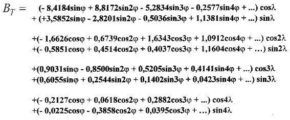 |
 |
The tesseral portion of the earth magnetic field. It is striking that all extreme values lie possibly at ±45 degree latitude. | |
| Illustration 9.10 - Tesseral part of the earth magnetic field |
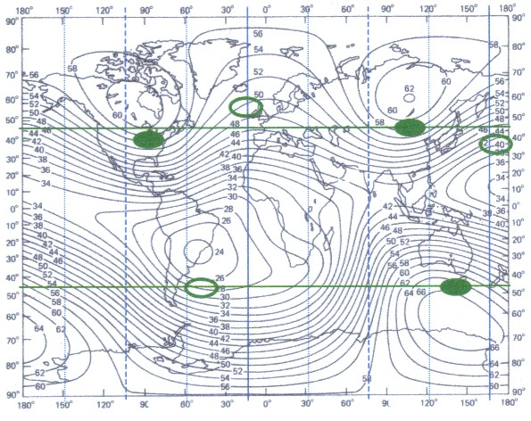
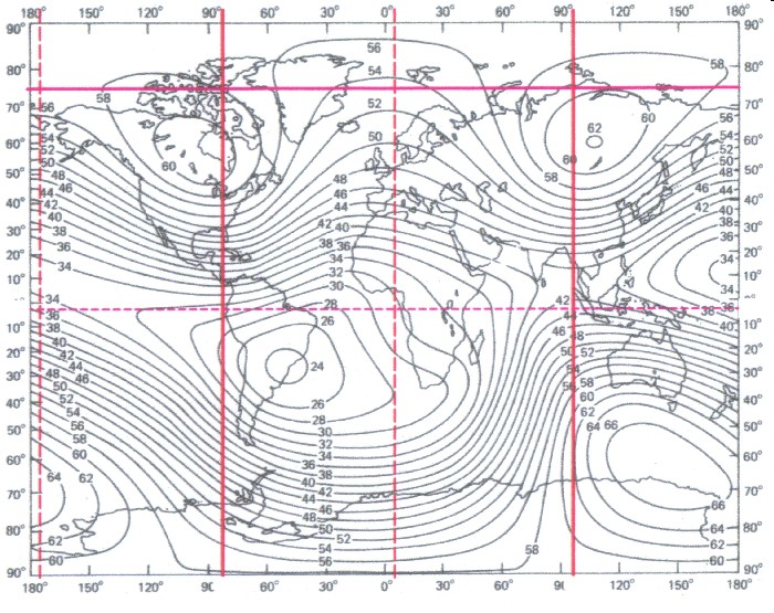
| If one marks the extreme values (green) of the tesseral part in a map with the total intensity and the axes for a three-axle ellipsoid (blue) with a 45-degree division, the following illustration 9.11 arises: |
|
| Illustration 9.11 - Tesseral extreme values of the earth magnetic field |
9.9 - The coordinates of the extreme values for the tesseral field
| The coordinates of the extreme values arise from the illustration 9.10: |
| Name | Latitude | Longitude |
| North-Maximum | +45 degrees of north | -95,7685 degrees of west |
| South-Maximum | -45 degrees of south | +129,21 degrees of east |
| Great Anomaly | +45 degrees of north | +99,7395 degrees of east |
| Minimum | -45 degrees of south | +8,395 degrees of west |
| On the north hemisphere all extreme values lie roughly on a square. A distorted cube or a spavin is generated according to co-ordinates in the earth by 45 degree latitude. |
| The book includes the illustrations 9.12 and 9.13 that deliver a polar representation of the tesseral field. |
![]()
| The book to the website - The website to
the book at time is the book only in german language available |
||
|
|
| The Advanced Book: Planetary Systems |
| The theory, which is developed in this book is based on the remake and expansion of an old idea. It was the idea of a central body, preferably in the shape of a ball, formed around or in concentric layers.
Democritus was the first who took this idea with his atomic theory and thereby introduced himself to the atoms as fixed and solid building blocks. Is the atom used as a wave model, that allows to interpret concentric layers as an expression of a spatial radial oscillator so you reach the current orbital model of atoms. Now, this book shows that these oscillatory order structures, described by Laplaces equation, on earth and their layers are (geologically and atmospherically) implemented. In addition the theory can be applied on concentric systems, which are not spherical but flat, like the solar system with its planets, the rings that have some planets and the moons of planets or also the neighbouring galaxies of the milky way. This principle is applicable on fruits and flowers, such as peach, orange, coconut, dahlia or narcissus. This allows the conclusion that the theory of a central body as a spatial radial oscillator can be applied also to other spherical phenomena such as spherical galactic nebulae, black holes, or even the universe itself. This in turn suggests that the idea of the central body constitutes a general principle of structuring in this universe as a spatial radial oscillator as well as macroscopic, microscopic and sub microscopic. |
|
![]()