|
|
| Impressum | Copyright © Klaus Piontzik | |
| German Version |
2 - The complete field of the earth
 |
The developed
approach in this book goes out from the complete field of
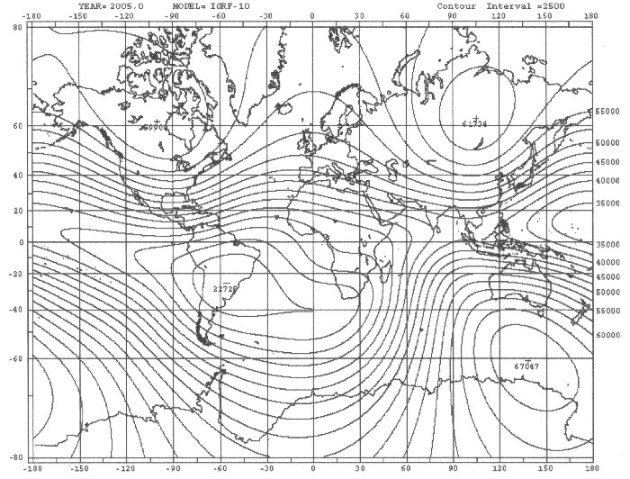
the total intensity of the earth. Hence, all following considerations and analyses are based on real, in the end measured values of the magnetic field. Here is a picture from the complete field of 1980, as it is published by various geophysical institutes as "International Geomagnetic Reference Field" briefly IGRF. You can find a table of the values here: Table of the earth magnetic field |
|
| Illustration 2.1 - The complete magnetic field of the earth - IGRF 1980 |
| Remarkably are the four extreme values of the field. (and not only two like the stick magnet or the dipole model) There are three maxima and one minimum. Also there exist one more saddle point (near Indonesia). |
| Here must be pointed out to the fact that, in the meantime, two models of the earth magnetic field exist, the IGRF and the WMM. |
| On the one hand, there is
the Internationally Geomagnetic Reference Field
briefly IGRF. Responsibly for the IGRF
are the "International Association of Geomagnetism
and Aeronomy" (IAGA), one of seven departments of
the IUGG (Internationally union of Geodesy and
Geophysics). The IGRF is made by hte V-8 IAGA Working Group which is responsible for "Analysis of the Global and Regional Geomagnetic Field and Its Secular Variation". The present 10th model bases on a revision from July, 1995 (XXI generals Assembly of the Internationally union of Geodesy and Geophysics in Boulder, Colo.) by the IGRF under addition of neighbouring models, which were provided by the NASA's "Goddard Space Flight Center", the "Institute of Terrestrial Magnetism, Ionospheric and Radio Wave Propagation" IZMIRAN as well as the U.S.Navy and the "British Geological Survey". The model is calculated for certenly 5 years and it is availible in the Internet. The valid model at time is the IGRF11 |
 |
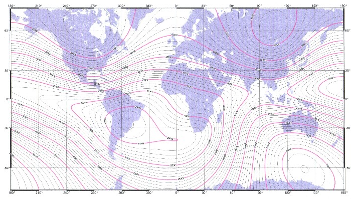
| Illustration 2.2 - The complete magnetic field of the earth – IGRF - 2005 |
| On the other hand one can
get the WMM 2005 about the "National Geophysical
Data Center" (NGDC), meanwhile also on the Internet.
The " World Magnetic of model "
(WMM) is a product of the U.S. National
Geospatial-Intelligence Agency (NGA). The NGDC and the British Geological Survey (BGS) made the WMM with support of the NGA in the USA, together with the "Defence Geographic Imagery" as well as the "Intelligence Agency" (DGIA) from Great Britain. The WMM is used as a standard model, for the US Department of Defense, the UK Ministry of Defence, the North Atlantic Treaty Organization (NATO), and the World Hydrographic office (WHO). It is widespread, in the meantime, also in the civil navigation. The model, the accompanying software and documentation are administered by the NGDC and the NGA. The model is made for 5 years in each case and the final date of the running model is 31th of December, 2009. The valid model at time is the WMM2010 |
 |
| Illustration 2.3 - The complete magnetic field of the earth – WMM - 2005 |
| The model valid at the moment, so the WMM 2005, is available under the title "The US/UK World Magnetic model for 2005-2010" as report NOAA Technical NESDIS/NGDC-1 from McLean, Macmillan, mouse, Lesur, Thomson and Dater since December, 2004 on the Internet. It contains the model with his mathematical derivations and also all relevant maps, like declension, inclination, vertical intensity etc. for the earth magnetic field. |
| In the book is
shown that the whole field structure has not
substantially changed during the last 300 years and the field of the complete intensity temporarily, for longer periods, so is virtually steady and it is for a general analysis of the earth field very well suitable |
| The Fourier analysis of the earth field will happen in detail in chapter 8 |
| The coordinates of the real extreme values can be determined in two ways. On the one hand, while one determines the edges of the extreme areas from Illustration 2.1 and forms from it the averages: |
The coordinates for the extreme values 1
| Name | Latitude | Longitude |
| North-Maximum | +56,8875 degrees North | - 96,125 degrees West |
| South-Maximum | -61,975 degrees South | +144,95 degrees East |
| Great Anomaly | +59,5375 degrees North | +107,125 degrees East |
| Minimum | -26,05 degrees South | - 50,8375 degrees West |
| Saddle point | +6,5 degrees North | +99,3125 degrees East |
The names of the extreme values come from geophysics and are usual there.
 |
The second
possibility of analysis consists in transferring the
complete intensities of the illustration 2.1 into a
numerical table (see here) in using these values for an analysis. This numerical use also permits a three-dimensional representation of the earth field. In the Illustration 2.2 the three maxima and the minimum can clearly be seen. |
|
| Illustration 2.2 - The intensity of the complete magnetic field of the earth by 3D view | ||
| From the invested table the co-ordinates of the extreme values can be determined: |
The coordinates for the extreme values 2
| Name | Latitude | Longitude |
| North-Maximum | +56,344 degrees North | - 96,04 degrees West |
| South-Maximum | -63,75 degrees South | +144 degrees East |
| Great Anomaly | +60 degrees North | +106,5 degrees East |
| Minimum | -26,25 degrees South | - 50,8145 degrees West |
| Saddle point | +7 degrees North | +99 degrees East |
| Iif one summarises both results, the areas arise in which the magnetic extreme values of the complete field lie. |
| Name | Latitude | Longitude |
| North-Maximum | 56,344-56,8875 degrees North | 96,04-96,125 degrees West |
| South-Maximum | 61,975-63,75 degrees South | 144-144,95 degrees East |
| Great Anomaliy | 59,5375-60 degrees North | 106,5-107,125 degrees East |
| Minimum | 26,05-26,25 degrees South | 50,8145-50,8375 degrees West |
| Saddle point | 6,5-7 degrees North | 99-99,3125 degrees East |
| Therefore four extreme values of the field arise with three maxima and a minimum. Besides there appears one more saddle point. These coordinates for the extreme values and extreme areas are furthermore in use and evaluation, in the still following investigations. |
| In 1838 Carl Friedrich Gauß determined the following potential equation for the earth magnetic field: |
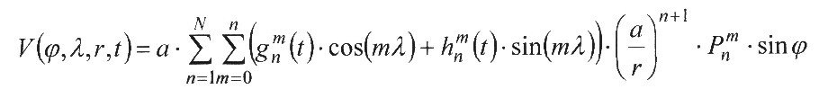 |
| Then the magnetic flux density B can be derived by using the gradient from the scalar potential field: |
 |
(see in addition also „ general theory of the geomagnetism “ from C.F.Gauß and W. Weber) |
| If one dissolves the brackets, merely products of sine or cosine functions appear in the equation by Gauß, so-called spherical harmonics. With those we will still occupy in chapter 5.3. |
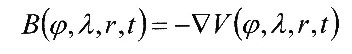
| The magnetic field of the earth is measured worldwide by more than 200 measuring stations. |
 |
| Illustration 2.8 - Measuring stations which are associated to the WMM-model |
| Since some decades the
field is also measured from satellites. The first
satellite was Magsat which registered in
1980 during six months the intensity and the complete
magnetic field. Since 1999 the danish satellite Ørstedt
is in an earth orbit and since July, 2000 the german
satellite Champ works. All appearing data above the earth magnetic field are collected by the IUGG or the IAGA and are evaluated. These values serve under others the basis for the production of the models IGRF and WMM. The maps and with thus the whole field are calculated in principle by using the equation by Gauß. However, besides, one goes and adapts the coefficients gn and hn to the multi-pole model !! However, this use of the equation by Gauß is problematic, because the dipole theory is still a part of consideration and use. An attempt which renounces the dipole model consists in taking the total intensities of the illustration 2.1 (or the accompanying table) and in using these values for an analysis. An entire analysis of the earth field can be managed by a two-dimensional Fourier analysis of the total intensities which will still occur in chapter 8. |
![]()
| The book to the website - The website to
the book at time is the book only in german language available |
||
|
|
| The Advanced Book: Planetary Systems |
| The theory, which is developed in this book is based on the remake and expansion of an old idea. It was the idea of a central body, preferably in the shape of a ball, formed around or in concentric layers.
Democritus was the first who took this idea with his atomic theory and thereby introduced himself to the atoms as fixed and solid building blocks. Is the atom used as a wave model, that allows to interpret concentric layers as an expression of a spatial radial oscillator so you reach the current orbital model of atoms. Now, this book shows that these oscillatory order structures, described by Laplaces equation, on earth and their layers are (geologically and atmospherically) implemented. In addition the theory can be applied on concentric systems, which are not spherical but flat, like the solar system with its planets, the rings that have some planets and the moons of planets or also the neighbouring galaxies of the milky way. This principle is applicable on fruits and flowers, such as peach, orange, coconut, dahlia or narcissus. This allows the conclusion that the theory of a central body as a spatial radial oscillator can be applied also to other spherical phenomena such as spherical galactic nebulae, black holes, or even the universe itself. This in turn suggests that the idea of the central body constitutes a general principle of structuring in this universe as a spatial radial oscillator as well as macroscopic, microscopic and sub microscopic. |
|
![]()