|
|
| Impressum | Copyright © Klaus Piontzik | |
| German Version |
1 - The dipole field of the earth
|
From the school, and from the media, we know
the magnetic field of the earth always as a field which
corresponds to the field of a rod magnet. It is the
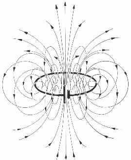
so-called dipole field. The physical attempt for such a magnetic field consists in the consideration of the magnetic field of a current loop. The mathematical derivation leads to a differential formula in which a so-called elliptical integral appears for which no closed mathematical solution exists - in form of an equation. |
|
| Illustration 1.1 - Current loop and dipole |
| The general proceeding consists in converting the appearing term in the integral into an infinite row. |
Simplified: |
| B = a1·x + a2·x2 + a3·x3 + a4·x4 + ... |
Then one goes and simply cuts off this row after the first limb. If one integrates now the left-over, the formula for the dipole field appears.: |
 |
| In the equation stands B for the
magnetic flux density, φ (phi) for the
latitude, m for the magnetic moment, r for
the earth radius and μ for the magnetic
permeability. m, r, μ are constants which are defined as follows: In this
case the magnetic moment is the magnetic moment of the
earth with m = 6,6845·1022
Am2 For the earth radius one takes the value from a geodetic system, in this case the WGS84 with: r = 6378155 m The magnetic permeability μ = 10-7 Vs/Am (For the derivation of the dipole field see also "Berkeley Physik Kurs 2" from Edward Purcell, page 266-269) |
| It is distinguished
between the magnetic poles and the geomagnetic
poles. The magnetic poles are the places in those
the magnetic field vertically stands on the earth
surface. The geomagnetic poles are the poles of the
dipole field. In the
geomagnetic poles the axis of the approximated dipole
field cuts the earth surface. First the dipole axis, so the geomagnetic poles, should be looked here. In older physics books you find often following values for the dipole axis (state in 1980): |
| Name | Latitude | Longitude |
| Dipole axis - North | +78,8 degrees North | -70,9 degrees West |
| Dipole axis - South | -78,8 degrees South | +109,1 degrees East |
| For the dipole axis one receives, in the popular-scientific literature, also the coordinates 79 degrees of north in latitude and 70 degrees of west in longitude. |
| In the book the at the moment counting dipole model which is based on the IGRF 1995 is still treated. |
| The dipole axis has tipped over, in comparison to physical axis of rotation, possibly about 11 degrees. This angle must be still taken into consideration in the above equation. If one uses the values of the constants, the following final formula arises for the magnetic flux density which is dependent practically only on the latitude: |
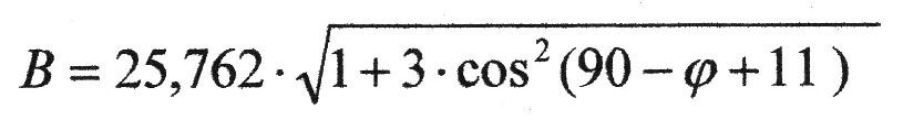 |
μT (mükroTesla) |
| Remark: 1 μT = 1000 γ (1 mükroTesla = 1000 Gamma) |
| The
mathematical approach shown here for reaching the dipole
equation can be looked on account of the cut-off rest
limbs, merely as a first approximation.
Particularly as still to be seen in the book, that the
dipole model is not constant in the course of time, in
its spatial position, and must be adapted. If one starts integrating the remaining limbs of the infinite row (from the current loop consideration), one receives the quadrupol field, the octupol field etc. |
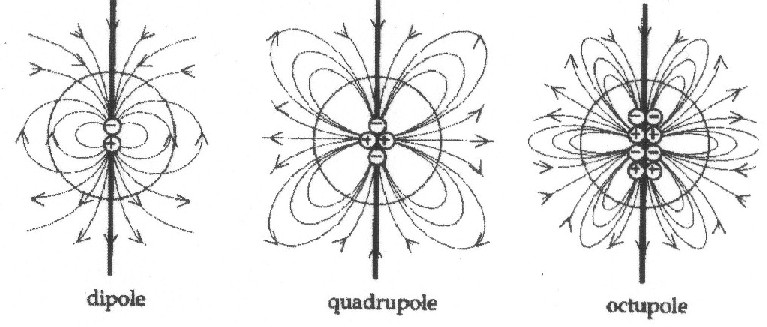 |
| Illustration 1.2 - The multi- pole development for the magnetic field |
| By changing the terms in
a row the whole process is an approximative, the solution
is only one approximation. In addition, is always to be
considered that the described approach is a purely
mathematical one. Besides, the question by
physical relevance stays open !!! If one takes actual values of the field, there can be shown, with the magnetic poles, that the dipole model is not enough to explain the earth magnetic field. |
| The field vector B of the earth magnetic field is described by three dimensions independent of each other which are called elements of the magnetic earth field. There exist two different systems of representation. Here only the system from Illustration.1.3 is shown and explained because of simplicity. |
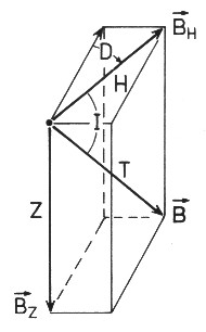 |
| Illustration 1.3 - Field elements of the magnetic field |
| The horizontal angle
between the direction from magnetic pole to the
geographic north pole is called declension
D or also horizontal magnetic variation. The horizontal
direction to the magnetic poles can be determined
directly with a compass. For the vertical deviation of the magnetic field vector of the parallel orientation to the earth surface the concept inclination I is used. If one so twists the compass so that its axis lies horizontal, we have an inclinatorium before ourselves - it misses the angle between the earth surface and the magnetic field. The fact that there is this angle and that it is depend of the measuring place is known for over 400 years. The fact that in the pole the magnetic field stands vertically on the earth surface and in the equator, however, in parallel with the earth surface has led with to the dipole model. And the vertical component of the magnetic field vector is called vertical intensity Z. (see also " Grundlagen der Geophysik " from Hans Berckhemer, page 138) |
| If one takes the "International Geomagnetic Reference Field" briefly IGRF of 1980 for the declension so the following illustration 1.4 arises (to the IGRF see also chapter 2.2) |
 |
By analysis of the declension, so of the
horizontal false variation of the earth
field, two areas can be won. Since the south and the
north-magnetic pole, the places in those the magnetic
field vertically on the earth surface stands and, hence,
exists here no horizontal variation. These both areas define the
magnetic poles. The inclination can be pulled up alternatively for the declension of course also to the pole determination. |
|
| Illustration 1.4 - The declension of the earth magnetic field - IGRF 1980 |
| The coordinates of the real poles can be found, while one determines the edges of the pole areas from illustration 1.4 and forms from it the averages: |
| Name | Latitude | Longitude |
| South-magnetic pole | +75 degrees North | -103,5 degrees West |
| North-magnetic pole | -65,5 degrees South | +141 degrees East |
| However, in physics books or in the popular-scientific literature one also finds the following coordinates: |
| Name | Latitude | Longitude |
| South-magnetic pole | +75 degrees North | -101 degrees West |
| North-magnetic pole | -67 degrees South | +143 degrees East |
| If one summarises both results, the areas in which the magnetic poles lie nowadays arise: |
| Name | Latitude | Longitude |
| South-magnetic pole | 75 degrees North | 101-103,5 degrees West |
| North-magnetic pole | 65,5-67 degrees South | 141-143 degrees East |
| In the book the at the moment counting pole areas (2005) are still treated. |
| If one
compares the found areas, from chapter 1.4 with the
coordinates of the dipole axis from chapter 1.2, one
recognises: 1) The pole areas do not subtend themselves as one would expect it after the dipole theory. 2) The available pole areas do not lie yet near the dipole axis. |
| From it two
possible conclusions can be drawn: 1) other influences must be here which disturb or distort the dipole field. The dipole model shows therefore only one partial view of the complete earth-magnetic field. The spatial change of the dipole axis in the course of time likewise speaks for it. 2) the dipole model does not fit here and one would have to keep a lookout after a new approach. The dipole model also does not last around to describe, the complete magnetic field of the earth with its four extreme areas in the next chapter. The result is: |
| The dipole model only is not
sufficient, to be able to explain the actual earth magnetic field. |
| And
with the multi-pole development of the earth field the
question by physical relevance stays open !!! Remark: Already Gauß and Weber recognised in 1838, by their experiments with the earth magnetic field that the magnetic field cannot be simply explained by the model of a stick magnet or a current loop. (see in addition also chapter 2.7) |
![]()
| The book to the website - The website to
the book at time is the book only in german language available |
||
|
|
| The Advanced Book: Planetary Systems |
| The theory, which is developed in this book is based on the remake and expansion of an old idea. It was the idea of a central body, preferably in the shape of a ball, formed around or in concentric layers.
Democritus was the first who took this idea with his atomic theory and thereby introduced himself to the atoms as fixed and solid building blocks. Is the atom used as a wave model, that allows to interpret concentric layers as an expression of a spatial radial oscillator so you reach the current orbital model of atoms. Now, this book shows that these oscillatory order structures, described by Laplaces equation, on earth and their layers are (geologically and atmospherically) implemented. In addition the theory can be applied on concentric systems, which are not spherical but flat, like the solar system with its planets, the rings that have some planets and the moons of planets or also the neighbouring galaxies of the milky way. This principle is applicable on fruits and flowers, such as peach, orange, coconut, dahlia or narcissus. This allows the conclusion that the theory of a central body as a spatial radial oscillator can be applied also to other spherical phenomena such as spherical galactic nebulae, black holes, or even the universe itself. This in turn suggests that the idea of the central body constitutes a general principle of structuring in this universe as a spatial radial oscillator as well as macroscopic, microscopic and sub microscopic. |
|
![]()