|
|
| Impressum | Copyright © Klaus Piontzik | |
| German Version |
15 - Magnetic layers and frequencies 1
15.1 - Distance consideration
| If one looks closer to the distances (from the distance table - chapter 12.2), one recognises they all form multiple of the radius R=6355758,426 m = Lo. This is the basic hull radius. So the distance values can be also shown so: |
| k | 1 | 2 | 3 | 4 | 5 | 6 | 7 | 8 | |
| n | m | ||||||||
| 1 | 1 | Lo | 3Lo | 5Lo | 7Lo | 9Lo | 11Lo | 13Lo | 15Lo |
15.2 - Frequency consideration
| If one understands the distances l' from the distance table as a wavelength of the accompanying hull respectivly of the oscillation layer, then frequencies can be also assigned to all distances. |
15.2.1 - Case 1
| A possibility exists to
orientate by the illustration 6.2. The double diameter is
equivalent to the wavelength. Then it is worth λ = 4R = 4l' and: |
 |
| The distance values for n=1 are used from the distance table for the following considerations. |
| k | 1 | 2 | 3 | 4 | 5 | 6 | 7 | 8 | ||
| n | m | |||||||||
| 1 | 1 | 11,79 | 3,93 | 2,358 | 1,68 | 1,31 | 1,07 | 0,907 | 0,786 | Hz |
| 6355,76 | 19067,28 | 31778,79 | 44490,31 | 57201,83 | 69913,34 | 82624,86 | 95336,38 | Km |
| It is to be noticed here that for k=2 the half Schumann frequency originates. |
15.2.2 - Case 2
| A farther possibility
exists to take the whole diameter of the accompanying
hull respectively of the oscillation layer as a
wavelength. So λ = 2R = 2l' and: |
 |
| From the distance table the distance values are used again for n=1. |
| k | 1 | 2 | 3 | 4 | 5 | 6 | 7 | 8 | ||
| n | m | |||||||||
| 1 | 1 | 23,584 | 7,861 | 4,716 | 3,369 | 2,62 | 2,143 | 1,814 | 1,572 | Hz |
| 6355,76 | 19067,28 | 31778,79 | 44490,31 | 57201,83 | 69913,34 | 82624,86 | 95336,38 | Km |
| It is to be noticed here that for k=2 the Schumann frequency originates. However, this signifies also that the Schumann frequency is already included in the spectrum of the earth-magnetic frequencies. All appearing frequencies are virtually doublings of the already found basic frequencies so explaining harmonics. |
15.2.3 - Case 3
| For the end here exist still the possibility to interpret the radius of the accompanying hull respectively of the oscillation layer as a wavelength. So λ = R = l' and: |
 |
| From the distance table the distance values are used again for n=1. |
| k | 1 | 2 | 3 | 4 | 5 | 6 | 7 | 8 | ||
| n | m | |||||||||
| 1 | 1 | 47,17 | 15,72 | 9,43 | 6,74 | 5,24 | 4,29 | 3,63 | 3,14 | Hz |
| 6355,76 | 19067,28 | 31778,79 | 44490,31 | 57201,83 | 69913,34 | 82624,86 | 95336,38 | Km |
| All appearing frequencies are virtually quads of the already found basic frequencies, shows merely harmonics. |
15.2.4 - Complete reflection
| All together the distance and frequency values can be shown for n=1 then as follows: |
| k | 1 | 2 | 3 | 4 | 5 | 6 | 7 | 8 | |
| n | m | ||||||||
| 1 | 1 | 3/2fS | 1/2fS | 3/10 fS | 3/14 fS | 1/6 fS | 3/22 fS | 3/26 fS | 1/10 fS |
| 1/f0 | 1/3f0 | 1/5f0 | 1/7f0 | 1/9f0 | 1/11f0 | 1/13f0 | 1/15f0 | ||
| Lo | 3Lo | 5Lo | 7Lo | 9Lo | 11Lo | 13Lo | 15Lo |
| The consequence is that all appearing frequencies in case 1 are representable as rational fraction multiples of certain basic frequencies. |
| In the book the table of the extreme layers from chapter 12.2 is transformed by the described allocation (case 1) to a frequency table. |
15.3 - Earth frequency and Schumann frequency
| If one looks closer to
the frequencies, a connection can be derived between
earth frequency and Schumann frequency. Easier this succeeds with the frequencies fH2. There exists since a common divisor frequency. |
| For k=1 and k=2 exists a
common divisor frequency with: 23,584 = 3 · 7,861 23,584 = 2 · 11,792 The frequency 7,861 Hz = fS corresponds to the Schumann freuqency Then the frequency can be disassembled for k=1, on the other hand, so: |
| 23,584 Hz =3fS = 2f0 |
| The general relation is (see chapter 15.2 - case 2): |
 |
| And from it directly deducible: |
 |
| The Schumann frequency is already included in the spectrum of the earth frequencies |
| From the equation for fH2 is also directly deducible: |
 |
| Furthermore directly deducible: |
 |
| The basic hull radius is only a little smaller then the pole or equator radius. Hence, the question arises here which dimensions fS owns if the hull radius is substituted with RA respectively. RP |
| The data of
the geodetic reference system WGS84 are: pole radius: RP= 6356752 m equator radius: RA= 6378137 m With c = 299792458 m/s as the speed of light arises for the single frequencies: |
||
| For the earth frequencies: | ||
| For the pole radius |  |
= 11,7899 Hz |
| For the equator radius |  |
= 11,7503 Hz |
| For the Schumann frequencies: | ||
| For the pole radius |  |
= 7,8602 Hz |
| For the equator radius |  |
= 7,8339 Hz |
| Noteworthy here is still
the fact that the Schumann frequency, for historical
reasons, is won from a cavity resonator consideration.
(see in addition chapter 7.1) The concurrent derivation from the earth frequency, so, in the end, from the radii of the earth, shows that the measurements of this planet and the generated frequencies on it stands in a closed connection. |
15.4 - An approximation for the equator frequencies
| If one takes, in the geophysical sciences usual, middle radius of 6,371 km, one receives for fS a value from 47,0558 hertz. This lies near with 47 hertz. |
| If one calculates on 47 hertz back, the radius arises to 6,378,563 km. This is about 400 metres bigger than the equator radius. Approximately one can say: |
| 47 Hz =6fS = 4f0 |
| From it arises: |
| fS = 47:6 Hz = 7,8333... Hz |
| f0 = 47:4 Hz = 11,75 Hz |
| This can be used as a good approximation for the equator radius frequencies. |
15.5 - Common frequencies
| A general connection can
be derived by the equation from chapter 15.3 still
between earth frequency and Schumann frequency. The relation f0/3 = fS/2 is preserved also if one multiplies the equation by a rational number, so to a fraction. With it arises in general: |
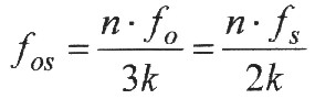 |
| n and k are elements of the natural numbers (1, 2, 3, 4...) |
| A complete spectrum of
common frequency fos originates from the equation, so
that the earth frequency and the Schumann frequency stand
with each other in a functional connection. Systematic using of the parametres n and k in the equation leads to a table in which then all common frequencies are included. The calculation of the table values occurs about the corrected basic frequency from chapter 11.2. A rounded value from fo = 11,792 Hz is used. |
common frequencies for n<17, k<9
| k | 1 | 2 | 3 | 4 | 5 | 6 | 7 | 8 | |
| n | |||||||||
| 1 | 3,9307 | 1,9653 | 1,3102 | 0,9827 | 0,7861 | 0,6551 | 0,5615 | 0,4913 | Hz |
| 2 | 7,8613 | 3,9307 | 2,6204 | 1,9653 | 1,5723 | 1,3102 | 1,123 | 0,9827 | Hz |
| 3 | 11,792 | 5,896 | 3,9307 | 2,948 | 2,3584 | 1,9653 | 1,6846 | 1,474 | Hz |
| 4 | 15,7227 | 7,861 | 5,2409 | 3,9307 | 3,1445 | 2,6204 | 2,2461 | 1,9653 | Hz |
| 5 | 19,6533 | 9,8267 | 6,5511 | 4,9133 | 3,9307 | 3,2756 | 2,8076 | 2,4567 | Hz |
| 6 | 23,584 | 11,792 | 7,8613 | 5,896 | 4,7168 | 3,9307 | 3,3691 | 2,948 | Hz |
| 7 | 27,5147 | 13,7573 | 9,1716 | 6,8787 | 5,503 | 4,5858 | 3,9307 | 3,4393 | Hz |
| 8 | 31,4453 | 15,7227 | 10,4818 | 7,8613 | 6,2891 | 5,2409 | 4,4922 | 3,9307 | Hz |
| 9 | 35,376 | 17,688 | 11,792 | 8,844 | 7,0752 | 5,896 | 5,0537 | 4,422 | Hz |
| 10 | 39,3067 | 19,6533 | 13,1022 | 9,8267 | 7,8613 | 6,5511 | 5,6152 | 4,9133 | Hz |
| 11 | 43,2373 | 21,6187 | 14,4124 | 10,8093 | 8,6475 | 7,2062 | 6,1768 | 5,4047 | Hz |
| 12 | 47,168 | 23,584 | 15,7227 | 11,792 | 9,4336 | 7,8613 | 6,7383 | 5,896 | Hz |
| 13 | 51,0987 | 25,5493 | 17,0329 | 12,7747 | 10,2197 | 8,5164 | 7,2998 | 6,3873 | Hz |
| 14 | 55,0293 | 27,5147 | 18,3431 | 13,7573 | 11,0059 | 9,1716 | 7,8613 | 6,8787 | Hz |
| 15 | 58,96 | 29,48 | 19,6533 | 14,74 | 11,792 | 9,8267 | 8,4229 | 7,37 | Hz |
| 16 | 62,8907 | 31,4453 | 20,9636 | 15,7227 | 12,5781 | 10,4818 | 8,9844 | 7,8613 | Hz |
| Besides, the first
smallest natural frequency is fo/3 = fs/2 =
3,9307 Hz that earth frequency and Schumann's
frequency own together. The table with the common frequencies also contains all harmonics of the Schumann frequency. With it the Schumann spectrum (from chapter 7) belongs to the frequency spectrum of the table 46. I.e. the whole Schumann spectrum can be derived from the earth frequency. |
15.6 - The sferic frequencies
| Another connection from the equation of chapter 15.5 arises if bigger n, so higher frequency, are looked: |
common frequencies for 1055<n<12673, k<9
| k | 1 | 2 | 3 | 4 | 5 | 6 | 7 | 8 | |
| n | |||||||||
| 1056 | 4150,784 | 2075,392 | 1383,595 | 1037,696 | 830,157 | 691,797 | 592,969 | 518,848 | Hz |
| 1584 | 6226,176 | 3113,088 | 2075,392 | 1556,544 | 1245,235 | 1037,696 | 889,454 | 778,272 | Hz |
| 2112 | 8301,568 | 4150,784 | 2767,189 | 2075,392 | 1660,314 | 1383,595 | 1185,938 | 1037,696 | Hz |
| 2640 | 10376,96 | 5188,48 | 3458,987 | 2594,24 | 2075,392 | 1729,493 | 1482,423 | 1297,12 | Hz |
| 3168 | 12452,35 | 6226,176 | 4150,784 | 3113,088 | 2490,47 | 2075,392 | 1778,907 | 1556,544 | Hz |
| 7128 | 28017,79 | 14008,89 | 9339,264 | 7004,448 | 5603,558 | 4669,632 | 4002,542 | 3502,224 | Hz |
| 12672 | 49809,41 | 24904,7 | 16603,14 | 12452,35 | 9961,882 | 8301,568 | 7115,63 | 6226,176 | Hz |
| The spectral maxima of
the sferic frequencies are given in general, as follows
in very much narrow-banded areas (see "Sferics" by Hans Baumer page 285): |
| 4150,84 Hz - 6226,26 Hz - 8301,26 Hz - 10377,10 Hz - 12452,52 Hz - 28018,17 Hz - 49810,08 Hz |
| The comparison of the
Sferic spectrum with the table values delivers a good
correspondence of the values. About the whole spectrum
seen the maximal mistake lies less than 0.7 hertz. In his book " the cosmic octave " (page 39) produces Cousto a connection between Sferic frequency and sidereal day. The comparison with the earth rotation delivers a minimum difference of about 3 hertz and grows with increasing frequency up to a maximum value of about 36 hertz. The increasing difference clearly shows that the frequency calculation about the sidereal day only is suited as an approximate value. As by the equation from chapter 15.5 and the generated table for 1055<n<12673 have been shown that the Sferic frequencies, with enough exactness, are included in the spectrum of the common earth frequencies and Schumann frequencies. |
![]()
| The book to the website - The website to
the book at time is the book only in german language available |
||
|
|
| The Advanced Book: Planetary Systems |
| The theory, which is developed in this book is based on the remake and expansion of an old idea. It was the idea of a central body, preferably in the shape of a ball, formed around or in concentric layers.
Democritus was the first who took this idea with his atomic theory and thereby introduced himself to the atoms as fixed and solid building blocks. Is the atom used as a wave model, that allows to interpret concentric layers as an expression of a spatial radial oscillator so you reach the current orbital model of atoms. Now, this book shows that these oscillatory order structures, described by Laplaces equation, on earth and their layers are (geologically and atmospherically) implemented. In addition the theory can be applied on concentric systems, which are not spherical but flat, like the solar system with its planets, the rings that have some planets and the moons of planets or also the neighbouring galaxies of the milky way. This principle is applicable on fruits and flowers, such as peach, orange, coconut, dahlia or narcissus. This allows the conclusion that the theory of a central body as a spatial radial oscillator can be applied also to other spherical phenomena such as spherical galactic nebulae, black holes, or even the universe itself. This in turn suggests that the idea of the central body constitutes a general principle of structuring in this universe as a spatial radial oscillator as well as macroscopic, microscopic and sub microscopic. |
|
![]()