Grids of the earth, grid structures of the earth

	The magnetic field of the earth Lattice structures of the earth magnetic field

Impressum	Copyright © Klaus Piontzik


German Version

11 - Global Grids / Planetary Grids

11.1 - Hartmann, Wittmann, Curry and Benker

At the beginning of the 50s Dr. med. Ernst Hartmann described an energetic grid system on the earth surface. Detailed experiments in addition can be found in the book "illness as a location problem". Hartmann spoke from a global grid, today it is better known under the name Hartmann-grid and is used in the radiesthesia, the building biology, the geobiology and also partially in the architecture. The so-called irritant stripes or -zones (stress stripe) of 20 cm width proceed in the magnetic north-south-direction in about 2 meter distance and in the east west direction with about 2.5 meter distance.

Another grid, earlier also diagonal grid called, was described between 1945 and 1951 by Siegfried Wittmann first. The actually known publication came in 1952 from Dr. Manfred Curry who did not mention the name Wittmann, however. Nowadays, hence, it is mostly simply called Curry-grid or also Curry-net. It proceeds from NE to SW and from NW to SE. Besides, the grid measure amounts to about 3.6 m x 3.6 m.

Anton Benker discovered in 1953 that the whole earth surface and the above lying space splits up in cubic fields with the distance of 10 meter. The Benker cube system (Benker cubical system) is generally seen, as a higher system to the Hartmann-grid.
(see in addition also „ radiology with the Benker cube system “ from Anton Benker)

The following generally relations are given:

In east-west direction: 1 Benker = 4 Hartmann
In North-South direction: 1 Benker = 5 Hartmann

11.1.1 - The attempt of Hartmann

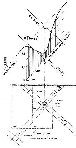		Picture 11.1 shows an experiment, that Hartmann carried out with a magnetic sensor (hall probe) in a cross point of the grid. The probe was moved once in the north-south and then in east-west-direction and, besides, the magnetic flux density was determined. In north-south- direction a clearly recognizable minimum is to be seen in the magnetic flux density. In east-west-direction the deviation is only minimal. (See in addition his book "illness as a location problem" page 457-Illustration 263) With his hall sensor experiment Hartmann has met the oscillation structure of the grid phenomenon without recognising, however, the consequences. If Hartmann was able to detect a minimum of the magnetic field, at the place of a cross point, the consequence is that here a row of minima exist – causes by the grid. Then between the minima, however, maxima also exist. And a sequnece of minima and maxima is an oscillation.
Illustration 11.1 - The experiment of Hartmann with a magnetic sensor

With his hall-probe attempt Hartmann has adduced the evidence for the connection of the grid phenomenon with the zonal part of the earth magnetic field.

Konsequenz:

There exist a relation between Hartmann-grid and the earth magnetic field

The consequence from the basic field model and the fourier analysis: the tesseral part of the earth magnetic field consists of basic fields, i.e. primarily of grid structures which are similar to the Hartmann-grid. The consequence is:

Grids are steady oscillation states of the earth magnetic field with certain frequency
There exist several lattice structures between which harmonical relations exist

11.1.2 - Curry-Benker connection

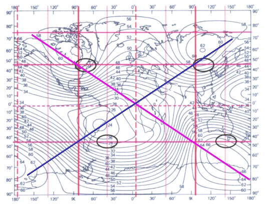The picture shows once more the ascertained huygens source areas of the tesseral field (black) with the magnetic main meridian (red vertically) from the sektorial part (or the grid ZS). See in addition chapter 9.

The blue and the magenta line show the theoretical (mathematical) connection between ideal source points if one applies the Huygens principle to the earth magnetic field.

The Benker-cube system (Hartman grid) is coupled with the earth-magnetic oscillation structure (red) in north south direction.

The curry net lies diagonally to the Benkersytem and with it in the level of the source connections (blue, magenta).

If one applies the basic field model to the Hartmann-grid and the Curry-grid, the following classification can be made:

The Hartmann-grid belongs to the basic fields
The Curry-grid lies in the plain of the basic oscillations

This permits the following approach: The curry net lies in the level of the basic oscillations and the Benkergitter is generated by the curry net. The approach occurs first in an Euclidean plain. Place of the consideration is the intersection of both generating oscillation levels.

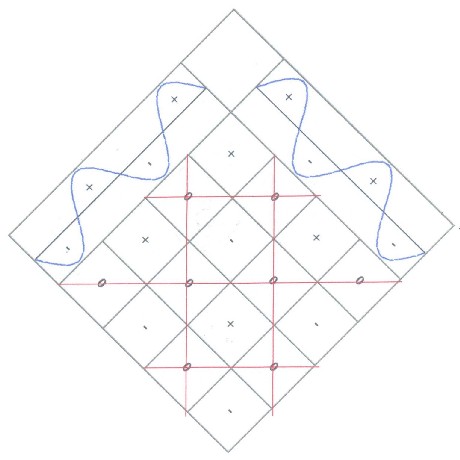		Starting point is the multiplication of two oscillations after chapter 5.4. Besides, the generated red grid should show the Benkersystem. The Benker grid is generated by the (blue) basic oscillations. It is worth: 1 basic oscillation = 1 Benker-diagonal
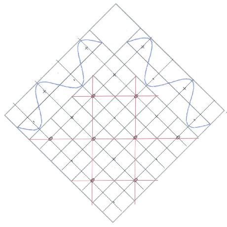		With ideal arrangement the curry net arises if the available zero grid is halved. Then it is worth (locally restrictedly): 1 Benker-diagonal = 4 Curry
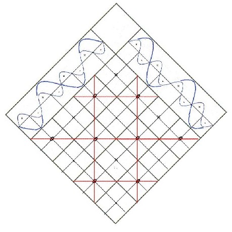		Halving of the zero grid means the double basic oscillation, so the first upper wave The curry net is the zero grid of the first upper wave

With ideal arrangement in an Euclidean plain the corner between curry net and Benkersystem arises always to 45 degrees. It is still to be considered that the whole grid production on a ball surface takes place. The corner is not steady there between curry net and Benkersystem, but is variable. All together from the geographic location dependent. Hence, on a ball surface Benker crossroads exist which do not any more collapse with the curry crossroads.

The curry net is the generating oscillation system
The curry net is the zero grid of the first upper wave of the basic oscillation

The Benker grid is generated by the basic oscillation
1 basic oscillation = 1 Benker-diagonal = 4 Curry

11.2 - basic hull and earth oscillation structure

As already in chapter 7.2 mentioned, the measurements which led to the discovery of the sferics took place between 1978 and 1979 in Pfaffenhofen at the Ilm. The basic frequency of the Sferics is declared with f = 4150,84 hertz. This value can be used to make a back calculation for the earth radius. The equation for the basic frequencies of the earth is:

formula for the basic frequencies of the earth

Change after R proves:

For n=1 the general equation for the earth radius is:

It is still to be taken into consideration that the sferic frequency of 4,150.84 hertz is the 11·2⁵ = 352-multiple of the basic frequency.

The basic earth frequency f₀ amounts to 11,79215909 Hz

With c = 299792458 m/s as the speed of light arises for the radius: R = 6355758,426 m = L_o
From now on this radius L_o is called: Basic hull radius

With this the oscillation structure can be defined for the earth:

Earth oscillation structure = sum of all possible space grids on the basic hull

11.2.1 - The stripe forming of the grid lines

Now the differences are formed between the data from a geodetic reference system and the calculated radius. (the basic hull)
The data of the geodetic reference system WGS84 are:

Pole radius : 6356752 m
Equator radius : 6378137 m

If one forms now the differences the following situation arises:

pole radius - basic hull radius = 993 m (about 1 km)
equator radius - basic hull radius = 22378 m (about 20 km)

The basic hull on that the zero lines and extreme values lie,
is between one and twenty kilometer
under the earth surface

And with thus an attempt is given to explain the stripe forming within the grids. Caused by the steady state, originate maximum fronts except also minimum fronts and zero fronts which spread spherically around the source points, and building regular intervals. Because the basic hull radius is smaller than the earth surface, so appear in the surface no lines but stripes. The following picture 11.2 illustrates the origin of the stripes on the earth surface.

Illustration 11.2 - The stripe forming by the basic oscillations

Therefore, the irritant stripes establish areas of decreased intensity, so no real zero zones.
As a consequence arises that a part of the irritant stripes, are not constant in their width, seen on a global scale. The stripes which virtually form the meridians of the oscillation system have their biggest width in the "equator" and become always narrow the "poles".
Merely the stripes which form the circles of latitude of the oscillation system, dispose of a constant width.

11.3 - To the Benker-Cube-System

At the same time an attempt which can explain the Benker-cube system arises by the radial components of the basic fields.
In the illustration 11.3 the oscillation situation is shown in the cross section and for one frequency. From the source points P going out, there arise, after the Huygens principle, around every source point concentric circles from minimum (red circles) - or maximum zones (blue circles). Because a steady state consists, the wave fronts are fixed in their spatial position.

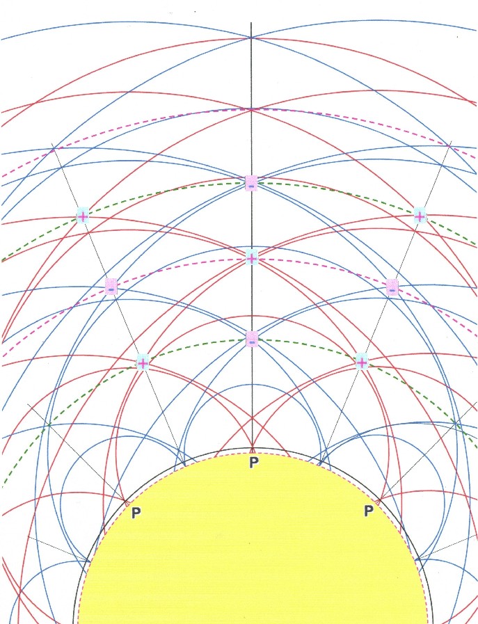Illustration 11.3 - Interferences of the basic oscillations

Oscillation maxima (with plus marked) and minima (with minus marked) originate from the interference of different wave fronts, indeed where several wave fronts establish an intersection respectively an area of concentration.
The so resulted oscillation extrema lie again on ball surfaces (dashed circles) which concentrically hull the earth.
It is noteworthy that a symmetrical configuration arises. There originates a spatial grid structure of extreme points which fills out the space around the earth completely. All plus and minus areas follow alternately on each other.

On the resulted spherical hulls maxima and minima arises. And like the basic fields (see chapter 5.5) there originate in addition the accompanying zero lines respective zero fronts.

		The single hulls (basic fields) are phases-moved to each other about 180 degrees. - And for this reason can originate between the extreme values now, in vertical (radial) as well as in tangential direction, whole zero surfaces. (magenta)

Illustration 11.4 - Spatial radial grid oscillations

These zero surfaces form the walls of a grid-shaped oscillation system and the extreme values are point-shaped in the centre of the in each case encasing ashlar.
To see likewise as in the illustration 11.4, the term cube system is not quite correct.

The Benker cube system is a spatial radial oscillation system with a grid structure

Besides, ground and covers surfaces are bent – it concerns parts of the spherical potential hulls. And the side walls are, because of the radial adjustment, also not parallel to each other. The whole can be called only in a first approximation cube system.
Subsequently all magnetic surface fields are to be understood as parts of the complete spatial oscillation system, because they are included as a respective oscillation layer in the whole.

All together appears that the basic fields (Hartmann-grid) and the radial grid-shaped oscillation system (Benker cube system) show not only two different sides of the same phenomenon,
but even cause themselves mutually.

11.4 - Global net grids (GNG)

Oscillation layers originate from the interference of magnetic waves with certain frequency producing suitable grid systems as steady states. I.e. however several grid systems can be formed here which differ merely by their frequency or their division relations.

Global net grids are steady spatial oscillation states of the earth magnetic field
Global net grids are connected with certain frequency


Because all these grids are based on integer limited numbers, so here it also comes to several division relations. In practice this means that several grids, in steady distances can overlap, in the irritant stripes. (zero zones)

With thus the derived model corresponds with the statements made in the radiesthesia about global net grid

Here must be pointed out once again to the fact that a complete square grid on a sphere cannot be realised. Really there exist only oscillation systems which are formed like the geographic grid system. There always exist two poles (which are not necessarily identical with the geographic Poles). The in each case accompanying "meridians" and "parallels" establish a grid system. From it also results that the grid squares are really square only in the "equator" of the oscillation system. These become to the poles more and more rectangles or rhombs and, in the end, at the pole one finds triangles.

11.4.1 - Shifting of irritant stripes
(Supplement to the symposium for geobiology 29.06.-01.07.2007 in Waldbrunn)

In the radiesthesian practise exist a row of observations which concern the phenomenon of a local or regional enduring shifting by irritant stripes. The grid model says the following:

	Subterranean objects (mineral resources, rejections(dismissals), magma bubbles) can lead locally or on a regional level to a shifting of the irritant stripes. Every bigger object has capazitive (plastics, earth) and/or inductive (metals) qualities. This can lead to a local or regional distortion of the grid.


In the radiesthesian practise exist a row of observations which concern the phenomenon of a temporary shifting by irritant stripes. The grid model admits here the following explanation:

The spatially radial grid system originates as an interference or as a sum of all basic oscillations – is so an oscillation system. Or physically expressed: the whole magnetic grid system is a harmonic oscillator. Strictly speaking even a damped harmonic oscillator. Besides, the grid walls are to be looked not as stiff but to see by the oscillation basis rather than energetic oscillation states. And with thus they are also variable in certain narrow borders. The consequence is: the grid system can produce in itself little oscillations which express themselves then in a position change of the irritant stripes. Besides, the irritant stripes swing to and fro. This applies in north-south-direction as well as in east-west-direction. However, these oscillations would ordinarily have to be so small that they are neglectable. Furthermore a light Pulsation of the whole system is also conceivable and with thus a light pulsation (in the width) of the irritant stripes is given.

Now, however, three cases would have to appear with temporarily recognizably bigger deviations of the irritant stripes.

In the first case can appear a deformation of the irritant stripes induced by geologic processes. The geologic layers are connected with magnetic layers (see chapter 13) and local geologic effects, like a small movement of tectonic plates respectively plate parts, can own a (elektro)magnetic equivalent. And these electromagnetic events can distort, as long as the geologic process lasts, the grid system locally or bring it also to oscillation.I

In the second case can appear, by solar influence, a global oscillation of the irritant stripes. Because also the atmospheric layers are connected with magnetic layers (see chapter 14), e.g., solar storms if they strike on the magnetosphere can bring the whole grid system in oscillation or lead to a temporary shifting of the irritant stripes.

In the third case can appear a temporary shifting of the irritant stripes induced by falling out of the solar influence, e.g. with a solar darkness.

In all three cases oscillation width of 1 meter can absolutely appear.

Now the following must be taken into consideration: The real generating elements of the earth magnetic field are magmatic streams at about 2,900-km depth. These streams are too sluggish to be impaired too strongly around by short-term geologic or solar events. Hence, the magnetic earth field and with thus also the magnetic grid system has a certain inertia. And this inertia acts against all external influences. Hence, one can understand the magnetic grid system also as a damped harmonic oscillator.
Besides, the system behaves like in the so-called „ aperiodic border case“. The resonance frequency and the frictional part of the oscillator keep, on this occasion, just the scales. Hence, it comes by an external effect on the oscillator to a unique reaction, in form of one swing. Then then the system returns slowly again in its resting state.

11.5 - A relation to the earth frequency

With the length data for the Hartmann grid or the Benker cube system and the basic field model a calculation is possible with which the accompanying grid frequency can be determined.
The Hartmann grid has about 2.5 meter of expansion in the east west direction. Four Hartmann fields fit in a Benker cube, so that the length of a cube arises to 10 meter.
However, according to the basic field model (chapter 5) two cubes (one positive and one negativ) generate an oscillation. For the wavelength arises 20 meter.
It is still to be considered that the used lengths are covered to the North European or German space. On average the 51 degree of latitude was accepted here. For the conversion at equator level the given distance must be divided by the cosine of the latitude. Thus arises for the wavelength a size of 31.78 meter in the equator. For the rest, 2513189 cubes fit thus round the earth, covered to the basic cover radius.
The general connection between wavelength and frequency is defined with: and the following f·? = c.
With ? = 31.78 m one receives the accompanying frequency:

f = 9433368,722 Hz.

If one examines the found frequency with the earth frequency fo=11,79215909 hertz from chapter 11.2 concerning the division relations, an amazingly easy prime factor decomposition is found:

11,792 · 2⁸ · 5⁵ = 11,792 · 800000 = 9433600

In general can be derived from the fact that the Benker-cube system swings in a frequency response of 9,433 - 9,434 MHz.

The Hartmann grid has the fourfold frequency, so 37,732 - 37,736 MHz in east west direction.

In north south direction five Hartmann fields fit in a Benker cube. Hence, still the frequency response 47,165 - 47.17 MHz appears with the Hartmann grid.

From it arises:

Hartmann grid and Benker cube system stand in relation to the earth frequency

11.6 - The source points of the earth field

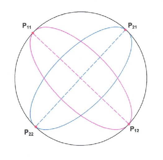
If one applies the basic field model from chapter 5 to the Hartmann-grid and the Curry-grid, the Hartmann-grid belongs to the basic fields. After the model the basic oscillations lie diagonally to the generated grid system. Therefore the Curry-grid lies in the plain of the basic oscillations.
If one looks now at a Hartmann field with both Curry diagonals so one can construct - by lengthening of the diagonals - on a sphere two circles, vertically on each other. See in addition picture 11.5. Now, however, can be taken, geometrically how physically, each of these both circles as a basic meridian of an oscillation system. And from it result two oscillation systems. What is for one system the main meridian is for the other system the equator. And both systems must harmonise in frequency and phase.

Two oscillation systems with four poles

Illustration 11.5 - Two oscillation systems with four poles

There form a total of four poles. There originate on the north hemisphere the both poles P₁₁ and P₂₁. On the south hemisphere there originate the accompanying poles P₁₂ and P₂₂. Then for symmetric reasons all poles lie on ± 45 degrees of latitude.
If one looks the whole field from chapter 2 in addition, there are really four extreme areas: the north maximum, the great anomaly, the south maximum and the minimum. The existence of the great anomaly beside the north maximum confirms here the existence of two oscillation systems. The consequence is:

There exist two basic oscillation systems (Curry-grids)
Both oscillation systems overlap mutually, because they stand vertically on each other

The magnetic back in the Arctic supplies here an other indication which originates from addition of the zonal with the sektoral part of the earth field. The magnetic back shows the maximum zone of the basic field ZS. (compares chapter 9.7) And it is also the direct connection between both northern Poles. If one lengthens this connection, the black full circle from picture 11.5 arises. Both oscillation systems have in common this circle. Hence, a main meridian of the complete system establish here. And exactly this is the maximum zone of the basic field ZS. The main meridian lies with Lambda = -83,5 degrees of west and Lambda = 96.5 degrees of east and is identical with the maximum zone of the grid ZS (respectively the sektoral field part).

The existence of a magnetic minimum admits even still an other conclusion: About the axis north maximum - south maximum (P₁₁ und P₁₂) a system with straight oscillations has been established. This means that in both Poles oscillation maxima are formed.

About the axis great anomaly - minimum (P₂₁ und P₂₂) a system from odd oscillations has been established. Of this fact results that in one pole an oscillation maximum is based and at the opposite end a minimum rules.

So then three maxima and a minimum originate from the sum forming of both systems.

With regard to the oscillation structure there are only three possibilities:

In the first case exist two straight basic oscillations - then there originate four maxima.
In the second case it appears an odd and a straight oscillation – then there originate 3 maxima and a minimum.
In the third case exist two odd basic oscillations – then there originate two maxima and two minima.

11.7 - The determination of the source points

In chapter 10.2 could be shown that virtually all magnetic extreme values - geographically according to length seen -fit in narrow areas. Practically all extreme values on the north hemisphere let themselves accommodate in a Zone of 55-90 west or 90-125 east. The extreme values on the south hemisphere can be arranged in a zone of 25-50 west or 130-155 east. Besides, the area on the north hemisphere is differently to the south hemisphere. The extreme zone on the north hemisphere is shifted about 35-40 degrees compared with the southern extreme zone.
This allows the suppose that both pole axis of the oscillation systems lie really not in a level how in illustration 11.5 are shown, but are shifted mutually. With it the pole axis also do not run through the centre of the earth.
Because it can be supposed that four poles are included in the extreme value areas like introduced in the chapter 10.2. With this the coordinates for the source points of the earth field can be found:I

Source point areas for oscillation system 1

Name	Breite	Länge
North-Maximum	+45° Nord	-55° bis 90° West
South-Maximum	-45° Süd	+130° bis 155° Ost

Source point areas for oscillation system 2

Name	Breite	Länge
Great Anomaly	+45° Nord	+90 bis 125° Ost
Minimum	-45° Süd	-25° bis 50° West

By average forming of the length areas, the coordinates of the source points are determinable:

Coordinates of source points for oscillation system 1

Name	Breite	Länge
North-Maximum	+45° Nord	- 72,5° West
South-Maximum	-45° Süd	+ 142,5° Ost

Coordinates of source points for oscillation system 2

Name	Breite	Länge
Great Anomaly	+45° Nord	+ 107,5° Ost
Minimum	-45° Süd	- 37,5° West

The basic field model and the Huygens principle (chapter 5) presumed, that these four poles are the theoretical source points which allow to build the whole external magnetic field of the earth.

11.8 - The B-Grid

if one puts down now all found magnetic extrema and points on a whole map of the complete intensity, illustration 11.6 arises:

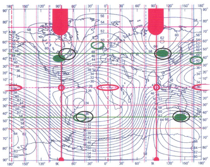Illustration 11.6 - All found magnetic extreme values and points

The blue lines show the axis of a three-axle ellipsoid, with a 45-degree division. The basic field ZS is shown red. All Green describes the tesseral field. And the black marks contain the source point areas.

The correspondence of the source point areas
with the four main extrema of the tesseral field is striking

The tesseral extrema are descended from the Fourieranalysis from chapter 8 to the 10, while the source point areas were won by an evaluation of the geographic length of all magnetic extrema in chapter 10. Because the tesseral field exists of grids, the source points (as a sum) are included in the lattice structures.

Well the main meridian of the complete system, so the maximum zone of the basic field ZS or the sektorial field part is also to be recognised with lambda =-83,5 degrees of west and lambda = 96.5 degrees of east.
On the north hemisphere are main meridian (and with it also the basic field ZS) in phase with the tesseral extreme values and the source point areas.
On the south hemisphere the tesseral extreme values or the source point areas are shifted about 20 degrees compared with the main meridian. What delivers a tip to the fact that there is in the internal earth structure a "sturgeon factor" which distorts the construction of a mathematically pure field.
If one puts down now all found magnetic extreme lines with the source point areas on a whole map of the complete intensity, illustration 11.7 or the B grid of the earth arises:

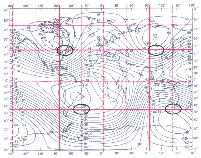Illustration 11.6 - The B-grid

The B grid contains all information of all appearing parts of the earth field. Well is to be recognised that all source point areas lie in phase to the main meridian at 83.5 degrees of west. This means that though the sturgeon factor shifts the earth field inside of the earth, however, this happens in harmony to the whole field.

There exist two possibilities to assign to the source point areas to a body in the interior of the earth: Either a spavin distorted about 35-40 degrees with only half of the corners is taken, or a Tetrahedron distorted about 35-40 degrees.

11.9 - Polyhedron

The single parts from the Fourieranalysis and all found magnetic extrema and points permit a stereometrical analysis and representation of the whole situation.

positions for the extrema of the grid ZS

In the map of the complete intensity all extreme values, magnetic structures and source points are put down, which arise by the analysis .

Blue – three-axle ellipsoid
Red – zonal, sektoal (grid ZS)
Green – tesseral
Black – source points

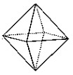
		The red magnetic system shows the grid ZS, so the zonal sektorial part. It becomes visible that a magnetic back on the North Pole originates, while in the South Pole only one point-shaped maximum zone exists. The maximum zone = magnetic main meridian (thickly red) is good to recognise, namely with &lambda =-83,5 degrees of west and &lambda = 96.5 degrees of east. The minimum zones (red sketched) lie with &lambda = 5.25 degrees of east and with &lambda =-174,25 degrees of west. In the equator-level there are two minimum zones and two saddle points. All extreme value zones lie on the corners of an octahedron

		The green system shows the tesseral part. All extreme values lie near ±45-degree latitude. The green points show the maximum points or minimum points of the pure grid part of the earth magnetic field. Full green = maximum, green bordered = minimum On the north hemisphere all extreme values lie roughly on a square. A distorted spavin (cube) is stretched according to coordinate in the earth by 45-degree latitude. The extreme zones on the south hemisphere are shifted about 35-40 degrees in longitude compared with the northern extreme zones.

		The black bordered ellipses are the source points of the whole field. The basic field or grid model and the Huygens principle presumed, show these four poles the theoretical source points from which the whole external magnetic field allows to stretch on the earth's surface. There is correspondence of the source point areas with the four main extrema of the tesseral field. The source points lie on the corners of a tetrahedron. The sources on the south hemisphere are shifted about 45 degrees

		With the help of the satellite geodesy in 1966 by C.A.Lundquist and G. Veis has been determined the following parametres to show the earth as a real three-axle ellipsoid: a₁-a₂ = 69 meter and &lambda₀ =-14,75 degrees of west The blue ellipsoid grid orients to the value of Lundquist and Veis is shifted to the red magnetic system about 1.25 degrees. Seen on a global scale a good correspondence is to be ascertained. The earth magnetic field stands in relation to the earth shape

An analysis for the geographic positions ofall appearing magnetic extrema proves a functional connection for their geographic length:

λ_E = m 3.75 ° – 13.5 °
3.75 ° by a 96th division, m is element of the integers

By the 96th division a sufficient differentiation exists to contain all appearing corners for polyhedron or the Platonic solids.

Consequence:

All Platonic solids are possible as oscillation figures

back

home

next

	The book to the website - The website to the book at time is the book only in german language available

buy on Amazon

in over 1000 Online Shops

Production and Publishing company:
Books on Demand GmbH, Norderstedt

ISBN 9-783833-491269

Store price: 35 Euro

380 sides
72 pictures of it 51 in colour
55 tables
1530 literature references
1900 entries in the register of names

The Advanced Book: Planetary Systems

The theory, which is developed in this book is based on the remake and expansion of an old idea. It was the idea of a central body, preferably in the shape of a ball, formed around or in concentric layers. Democritus was the first who took this idea with his atomic theory and thereby introduced himself to the atoms as fixed and solid building blocks.
Is the atom used as a wave model, that allows to interpret concentric layers as an expression of a spatial radial oscillator so you reach the current orbital model of atoms.
Now, this book shows that these oscillatory order structures, described by Laplace’s equation, on earth and their layers are (geologically and atmospherically) implemented. In addition the theory can be applied on concentric systems, which are not spherical but flat, like the solar system with its planets, the rings that have some planets and the moons of planets or also the neighbouring galaxies of the milky way. This principle is applicable on fruits and flowers, such as peach, orange, coconut, dahlia or narcissus.
This allows the conclusion that the theory of a central body as a spatial radial oscillator can be applied also to other spherical phenomena such as spherical galactic nebulae, black holes, or even the universe itself. This in turn suggests that the idea of the central body constitutes a general principle of structuring in this universe as a spatial radial oscillator as well as macroscopic, microscopic and sub microscopic.

buy on Amazon