|
|
| Impressum | Copyright © Klaus Piontzik | |
| German Version |
17 - The figure of the earth
17.1 - Geodetic systems
| Geodetic systems explain approximation models of the earth figure. Originate from a rotation ellipsoid such systems try to define the parametres which permit a more and more precise description of the earth in her 3-dimensional expansion. | ||
 |
Starting
point is normally an ellipsis with the great half-axis a
(major axis) and the small half-axis b
(minor axis). If one lets now the ellipsis rotate around
the smaller axis, there originates a so-called rotation
ellipsoid which is also called spheroid. However, with enough high exactness of the observation, turns out that an earth model based on an ellipsoid is not enough for an exact solution. |
|
| Illustration 17.1 - Origin of a rotation ellipsoid | ||
| The figure
of the earth is described by a physical and by a
mathematical surface. One understands the physical earth
surface as the limitation between hard and liquid earth
masses against the atmosphere. Here a density jump takes
place, so to speak, in the construction of the earth,
namely from the middle density of the upper earth crust
with r = 2,7 gcm-3 on the air density with r = 0,0013
gcm-3. However, the
irregularly formed surface of the hard earth masses, as
for example the continents, cannot be shown by a
mathematical relation. Nevertheless, the surface
of the oceans which amount at least about 70% of the
earth surface shows a forming law. Under certain
preconditions the seas establish a surface on which a
constant gravity potential exists. Then it is a level
surface of the earth gravity field. |
|
| Illustration 17.2 - Geoid |
| The earth is constructed
from masses of different density, however, which are not
steadily called homogeneous distributed. Hence, it can
seem locally that the physical (measured) plumb line
direction does not agree with the ellipsis-normal. These
plumb line divergences must be taken into the
consideration. These divergences are called geoid undulations. Hence, a reference ellipsoid is taken, normally, and the appearing heights above the ellipsoid surface are applied. |
| With the geoid determinations effected till this day has appeared that the divergences of the geoid from a middle rotation ellipsoid amount smaller than 100 metres by height. |
 |
To receive
one, still better adaptation to the geoid than a biaxial
rotation ellipsoid, would be seen geometrical, the next
step to try with a three-axle ellipsoid. In the
illustration 17.3 such an ellipsoid is shown. Referred to the earth then is a1, besides, the great equator half-axis, a2 the small equator half-axis and b the pole axis. |
|
| Illustration 17.3 - Three-axle ellipsoid | ||
| Attempts
have been started several times to determin the
parametres for a three-axle ellipsoid as an earth model. Nevertheless, the results are of each other different, namely because of the different distribution of the observations on the earth surface and the different methods by the reduction to the ellipsoid. |
| With the help of the satellite geodesy, in 1966 by C.A.Lundquist and G. Veis, the following parametres have been determined: |
| a1-a2
= 69 Meter λo = -14° 45` (longitude West) |
| Besides, a1 is the great equator half-axis, a2 the small equator half-axis and λo the longitude of the great
half-axis. If one takes now the value of Lundquist and Veis, and compares this to the zero point (-13,5 degrees longitude position - chapter 4 - angle approach) so can be ascertained, seen on a global scale, a good correspondence. |
| Because
the divergences of the biaxial rotation ellipsoid to the
geoid, lie normally, in the same scale like the axis
difference of 69 metres, a substantially better
adaptation to the geoid is not really reached by a
three-axle ellipsoid. On the other hand, however geodetic calculations are quite complicated by a more complex geometry of the ellipsoid. Also as a geophysical normal figure the three-axle ellipsoid is worse suitable, because with the values of the earth mass and the angular speed of the earth an unnatural form arises. Hence, the three-axle ellipsoid has not asserted as a relation body in the today's geodesy. |
| Strictly speaking rank the middle
rotation ellipsoid or the geoid and the
three-axleellipsoid, with regard to the divergences of
the actual earth figure, in the same scale. They are according to also equivalent models. |
17.2 - The average points of the earth
| If one
evaluates all averages which are possible in an ellipsis,
with regard to the axes, five cases arise. These are listed in the following table. Besides, the values are rounded, because all averages deviate merely a few arc seconds or arc minutes from the given numerical values. Besides, the kind of the average forming is arbitrary. Hence, it is not distinguished here any more between the single averages, but the averages are called in general with M. |
| CASE | Average condition | Angle |
| I | R=M | 45° |
| II | y=M/2 | 30° |
| III | x=M/2 | 60° |
| IV | x=M | 3° |
| V | y=M | - |
| Remarkable is that for y=M no averages exist, because all averages are greater than the small half-axis and lie, hence, beyond the ellipsis. If one marks all existing averages in the ellipse, the following illustration 17.4 arises: |
 |
| Illustration 17.4 - Ellipsis and her averages |
| If one takes
as an earth model a rotation ellipsoid,
the averages from the picture prove specific
circles of latitude. If one takes a three-axle ellipsoid as an earth model (values of Lundquist and Veist), single points arise. These points are called from now average points.If one puts down all average points on a drawing of the earth, the next picture arises: |
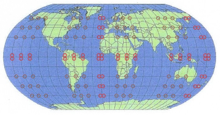 |
| Illustration 17.5 - Earth and average points |
| Only in
German language: A geodetic consideration of the average points can be looked up under "Die Gestalt der Erde-13" A derivation of the average points can be checked under "Die Gestalt der Erde-12" |
| A part of the
average points of the earth dispose of an astonishing
relation with the water course of the earth. Water occurence can be found in the following average points: South America - Amazon basin, North America - Ontario lake, Northern Europe - Ladoga lake, Africa - Victoria lake, Asia - Chanka lake, Australia - two areas with several lakes. The most important river deltas, which lie on average points are: Po delta, Danube delta and Volga delta in Europe and directly under it the Nile delta and the Euphrates/Tigris delta. As well as in South America Rio de la Plata and Amazon delta, in North America the Hudson Bay and in Asia the Yangtse delta. Furthermore are associated in Europe the Adriatic Sea, the Black Sea and the Caspian Sea with average points, as well as the Bottnisch bay. The position of the Mediterranean Sea between the average points is interesting also. Between two average points Baikal lake also lies in Asia. |
| The river deltas supply here virtually the answer. Because water always flows downwards, the river deltas must lie lower than the surrounding area. And this signifies: |
| The average points are, with regard to the land masses, the lowest points on the earth surface. |
17.3 - Magnetic field and average points
| Here the
positions of the magnetic extreme values from chapter
2 still interests
with regard to the average points. And this leads to the
next drawing 17.6. The magnetic central areas of the
extreme values for the complete field are yellow marked
here and the real extreme values are bordered in red. How to see the magnetic extreme values appear only in the edges of the average areas. And all extreme values lie on so-called specific circles of latitude (red lines) which arise from the osculating circle construction and the accompanying harmonious means of the ellipsoid axes. The osculating circles play a special role with the ellipsis. On the one hand the ellipse can be constructed with them relatively fast. On the other hand, the radii of the osculating circles, especially the smaller radius, are used to describe the ellipsis in her properties, e.g., for the ellipse as a conic section. Starting from a rotation model for the earth, is called from an arbitrary geodatic system, four specific circles of latitude originate from the osculating circle construction. |
| φ12
= ±29° 58' 19-20,5" φ34 = ±59° 58' 19-20,5" |
| Within the borders of 19-20,5 arc seconds there lie the values of all known geodetic systems. |
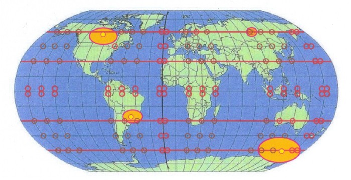 |
| Illustration 17.6 - Earth, average points and magnetic extreme values |
| The magnetic extreme values appear only in the edges of the average areas. And all extreme values lie on the specific circles of latitude (red lines) which arise from the osculating circle construction and the harmonious means. |
| The harmonious means of the ellipsoid axes take a special position with regard to the ellipse. There exists a relation with the osculating circle construction which here, however, is not entered closer. Two other specific circles of latitude originate from the harmonious means of the ellipsoid axes: |
| φ56 = ±30° 08' 17,6-24,5" |
| φ56 and
φ12 lie only 10 arc minutes apart and
cannot be distinguished with a global representation
(like in illustration 17.6) any more. Within the borders of 17,6-24,5 arc seconds there lie the values of all known geodetic systems. |
| Only in
german language: see in addition: "Die Gestalt der Erde-10" and "Die Gestalt der Erde-11" |
| From the drawings and the considerations the following conclusion can be drawn when one lays on a three-axle ellipsoid: |
| The positions of the magnetic extreme
values of the complete field stand in relation to the average points and the specific circles of latitude |
17.4 - Magnetic field and three-axle ellipsoid
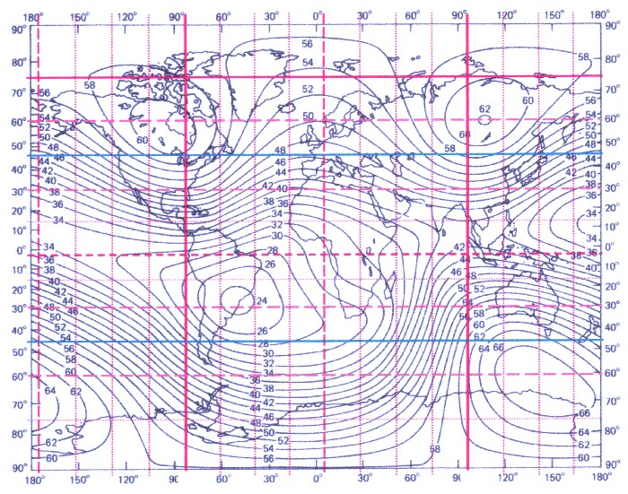
| If one puts down now all
found magnetic extreme values and points, as well as the
specific circles of latitude, in a whole map of the
complete intensity, arises illustration 17.7 which
virtually shows an extension of picture 11.6. The blue verticals in picture 17.7 show the axes of a three-axle ellipsoid, with a 22.5 degrees partition. The red verticals orientate themselves by the main meridian of the magnetic oscillation system, likewise with a 22.5 degrees partition. Well to be seen is that ellipsoid system and magnetic system differ only slightly of each other, lie so, so to speak, in phase to each other. The main axis of the three-axle ellipsoid lies, with Lundquist and Veis, at -14,75 degrees of west. The main meridian of the magnetic system lies at -83,5 degrees of west. A difference of 1.25 degrees arises from it between both systems. It is also the difference between the value of Lundquist and Veis, and the zero point from chapter 4. Seen on a global scale both systems agree therefore well. |
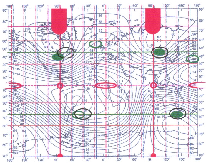 |
| Illustration 17.7 - Magnetic field and three-axle ellipsoid |
| Then from the drawing 17.7 the following conclusion can be drawn: |
| The
positions of all magnetic extreme values of the earth stands in relation to a three-axle ellipsoid |
| From the drawings 17.5 to 17.7 from these chapter and the previous considerations, primarily from the chapter 4.4, chapter 9.5 and chapter 13, the following conclusion can be drawn when one lays on a three-axle ellipsoid: |
| The
positions of all magnetic extreme values of the earth stands in relation to the figure of the earth |
17.5 - The C-grid
| Based on the 4-structure
of the sektoral part, a partition of 22.5 degrees (chapter
9) originates
round the equator. Caused by the specific circles of latitude and the 45 degrees of latitude from the tesseral system respectively the source points, a 15 degrees partition arises from north to south. With it the existing B-grid can be refined. If one draw in all latitudes and longitudes of both partitions 15 and 22.5 degrees, the C-grid appears: |
 |
| Illustration 17.8 - The C-grid |
| The C grid contains therefore all information above the magnetic field and about the earth figure, taking into account a three-axle ellipsoid. |
17.6 - The Bermuda triangle
| Since the appearance of
the books "the Bermuda triangle" in 1974/75 and
"Without a trace" in 1977 from Charles
Berlitz, numerous rumours have entwined
themselves round the phenomena, which have achieved
attention also in the wider public. The Bermudas triangle lies in the Atlantic sea area to the east of the peninsula of Florida. |
 |
| Illustration 17.9 - The Bermuda triangle |
| The results of the
magnetic field investigation of the author produced
knowledge which allows a statement to one of the
phenomena of the Bermuda triangle. Namely about the cases
described up to now of mysterious compass
behaviour like gyrating or swaying the compass
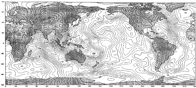
needle or also static magnetic variation. If one compares the position of the Bermuda triangle to the C-grid (illustration 17.8) so one recognises immediately that the triangle lies directly at the main meridian (λ =-83,5 degrees of west) of the planetary magnetic oscillation system. Because round the main meridian the extreme zone expands up to 15 degrees on both sides, the Bermuda triangle lies in the magnetic maximum zone of this planet. At the same time the 30th degree of latitude also proceeds through the area, and how in chapter 17.3 was to be seen, two geometrically specific circles of latitude lie here. (see also illustration 9.2, 9.5, 9.8 in chapter 9) If one pulls up now the map of the annual magnetic change (illustration 17.10) from the WMM 2005 ("World Magnetic Model" see also chapter 2) and marks the main meridian (with his maximum zones) of the planetary magnetic oscillation system, an amazing correspondence arises: |
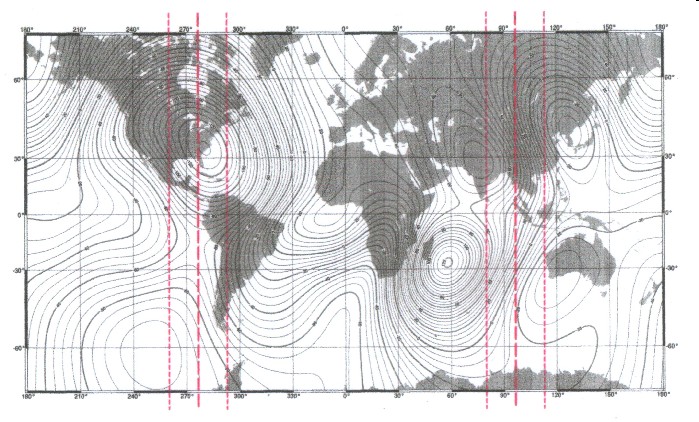 |
| Illustration 17.10 - Map of the annual magnetic change with main meridian - WMM 2005 |
| Only two
areas exist with a maximum in change of
the field. An area lies to the east of the
southern tip of Africa, the other area partially
corresponds with the Bermuda triangle. If one compares illustration 17.10 to illustration 17.7 or 17.8 so one recognises that the north maximum of the tesseral field and also a source point area are in immediate nearness (see also illustration 9.11in chapter 9). Because also the main meridian of the planetary oscillation system runs here, the consequence is that the Bermuda triangle is to be looked as the only place on the earth at which the strongest fluctuations can appear in the magnetic field. These fluctuations can appear temporarily as variations, as well as vary in the intensity and in the direction of field parts. Effects like gyrating or also swaying to a compass needle as well as static magnetic variation can be looked here as absolutely plausible. And this is exactly the kind of compass phenomena about which is reported that they appear in the Bermudas triangle. (see double book „The Bermuda triangle“ from Berlitz and Valentine, page 19, 24, 35, 73, 76, 77, 80, 91, 92 respectively "Without a trace", page 16, 17, 24, 25, 30, 46) |
![]()
| The book to the website - The website to
the book at time is the book only in german language available |
||
|
|
| The Advanced Book: Planetary Systems |
| The theory, which is developed in this book is based on the remake and expansion of an old idea. It was the idea of a central body, preferably in the shape of a ball, formed around or in concentric layers.
Democritus was the first who took this idea with his atomic theory and thereby introduced himself to the atoms as fixed and solid building blocks. Is the atom used as a wave model, that allows to interpret concentric layers as an expression of a spatial radial oscillator so you reach the current orbital model of atoms. Now, this book shows that these oscillatory order structures, described by Laplace`s equation, on earth and their layers are (geologically and atmospherically) implemented. In addition the theory can be applied on concentric systems, which are not spherical but flat, like the solar system with its planets, the rings that have some planets and the moons of planets or also the neighbouring galaxies of the milky way. This principle is applicable on fruits and flowers, such as peach, orange, coconut, dahlia or narcissus. This allows the conclusion that the theory of a central body as a spatial radial oscillator can be applied also to other spherical phenomena such as spherical galactic nebulae, black holes, or even the universe itself. This in turn suggests that the idea of the central body constitutes a general principle of structuring in this universe as a spatial radial oscillator as well as macroscopic, microscopic and sub microscopic. |
|
![]()